tryCatch({
  data(montreal.bikes, package="animint2")
}, warning=function(w){
  devtools::install_github("animint/animint2")
  data(montreal.bikes, package="animint2")
})9 Vélos de Montréal
Dans ce chapitre, nous explorerons plusieurs visualisations des données pour un ensemble de données portant sur les vélos de Montréal.
Plan du chapitre :
- Nous commençons par quelques séries temporelles non interactives.
- Nous créons une visualisation interactive de la fréquence des accidents dans le temps.
- Nous créons une visualisation interactive des données avec quatre graphiques, montrant les tendances mensuelles des accidents, les détails quotidiens et une carte des emplacements des compteurs.
9.1 Graphiques statiques
Nous commençons par charger le fichier montreal.bikes qui n’est pas disponible dans la version CRAN de animint2, afin d’économiser de l’espace sur le CRAN. Par conséquent, pour accéder à ce jeu de données, vous devrez installer animint2 depuis GitHub :
Les données sont deux séries temporelles :
-
montreal.bikes$counter.counts: les passages de vélos sur les compteurs, dans un tableau avec une ligne pour chaque combinaison de lieu et jour. -
montreal.bikes$accidents: les accidents, dans un tableau avec une ligne par accident.
Nous allons calculer des résumés par mois dans ces deux séries temporelles.
9.1.1 Compteurs
Pour commencer, nous affichons le tableau de données des compteurs de vélos.
mois_str <- function(POSIXct)strftime(POSIXct, "%Y-%m")
library(data.table)
(passages_dt <- data.table(montreal.bikes$counter.counts)[, .(
  lieu = location,
  date,
  mois.str = mois_str(date),
  passages=count)])
lieu date mois.str passages
1: Berri 2009-01-01 05:00:00 2009-01 29
2: Berri 2009-01-02 05:00:00 2009-01 19
---
13382: Totem_Laurier 2013-09-17 04:00:00 2013-09 3745
13383: Totem_Laurier 2013-09-18 04:00:00 2013-09 3921Ci-dessus, nous voyons une ligne pour chaque combinaison de lieu et jour. Le comptage de vélos présente des données de séries temporelles que nous visualisons ci-dessous.
passages_dt[, lieu.lines := gsub("[- _]", "\n", lieu)]
library(animint2)
ggplot()+
  theme_bw()+
  theme(panel.margin=grid::unit(0, "lines"))+
  facet_grid(lieu.lines ~ .)+
  geom_point(aes(
    date, passages, color=passages==0),
    shape=21,
    data=passages_dt)+
  scale_color_manual(values=c("TRUE"="grey", "FALSE"="black"))
Warning: Removed 407 rows containing missing values (geom_point).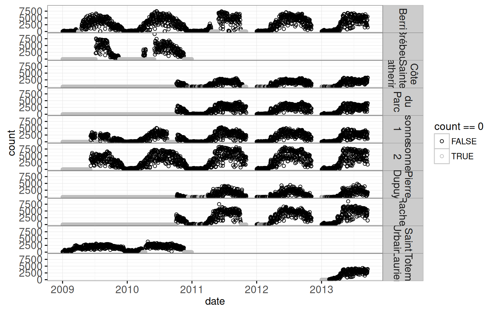
Le graphique ci-dessus données permet de voir facilement la différence entre les zéros (en gris) et les valeurs manquantes. On voit bien la régularité au fil des saisons (moins de vélos en hiver).
9.1.2 Accidents
Pour commencer avec les données d’accidents, nous affichons une ligne :
montreal.bikes$accidents[1,] date.str time.str deaths people.severely.injured people.slightly.injured
1 2012-01-02 18:35 0 0 1
street.number street cross.street location.int position.int
1 NA ST JEAN BAPTISTE O AV ROULEAU 32 6
position location
1 Voie de circulation En intersection (moins de 5 mètres)Pour chaque accident il y a des données sur la date, l’heure, la localisation et le nombre de morts et de blessés. Certaines valeurs sont en français (par exemple : Voie de circulation, En intersection, etc). Pour les colonnes avec noms en anglais, nous allons faire des copies en français :
gravité <- c(
  décès="deaths",
  grave="people.severely.injured",
  mineure="people.slightly.injured")
montreal.bikes$accidents[, names(gravité)] <-
  montreal.bikes$accidents[, gravité]
accidents_dt <- data.table(montreal.bikes$accidents[, c(
  "date.str", "time.str", names(gravité),
  "street", "street.number", "cross.street")])
Dans le code ci-dessous, nous rajoutons une colonne pour le mois.
ymd2POSIXct <- function(date.str){
  as.POSIXct(strptime(date.str, "%Y-%m-%d"))
}
(accidents_dt[
, date := ymd2POSIXct(date.str)
][
, mois.str := mois_str(date)
][])
date.str time.str décès grave mineure street street.number
1: 2012-01-02 18:35 0 0 1 ST JEAN BAPTISTE O NA
2: 2012-01-05 21:50 0 0 1 FOSTER NA
---
5594: 2014-12-27 12:35 0 0 1 CH DES PATRIOTES NA
5595: 2014-12-30 11:55 0 0 1 PIERREFONDS BD 14965
cross.street date mois.str
1: AV ROULEAU 2012-01-02 2012-01
2: JANELLE 2012-01-05 2012-01
---
5594: 1RE RUE 2014-12-27 2014-12
5595: JACQUES BIZARD 2014-12-30 2014-12Dans la sortie ci-dessus, on voit que les derniers mois pour les accidents ne sont pas les mêmes que les compteurs. On compare les intervalles dans le code ci-dessous :
     accidents passages
[1,] "2012-01" "2009-01"
[2,] "2014-12" "2013-09"
Dans la sortie ci-dessus, on voit que les passages et les accidents se chevauchent. Nous allons compiler des résumés pour tous les mois, c’est pourquoi nous faisons un tableau de données pour chaque mois ci-dessous.
Le code ci-dessous définit l’environnement linguistique (locale) pour avoir les noms de mois en français.
old.locale <- Sys.setlocale(locale="fr_CA.UTF-8")
mois_français_str <- function(POSIXct)strftime(POSIXct, "%B %Y")
mois.levs <- mois_français_str(mois_dt$mois.01)
mois_français <- function(POSIXct)factor(
  mois_français_str(POSIXct), mois.levs)
mois_dt[, mois.français := mois_français(mois.01)][]
mois.01 mois.français
1: 2009-01-01 janvier 2009
2: 2009-02-01 février 2009
---
71: 2014-11-01 novembre 2014
72: 2014-12-01 décembre 2014La sortie ci-dessus comprend une ligne pour chaque mois. Notez que nous avons créé une colonne mois.français qui sera utilisé comme variable de sélection pour les mois. Dans le code ci-dessous, nous calculons la somme des accidents par mois.
    mois.str décès grave mineure
 1:  2012-01     1     0      10
 2:  2012-02     0     0      20
---
35:  2014-11     1     2      69
36:  2014-12     0     0      10
Ci-dessus on voit une ligne pour chaque mois, avec différentes colonnes pour chaque niveau de gravité. Nous convertissons ces colonnes en lignes avec le code ci-dessous :
     mois.str gravité personnes
  1:  2012-01   décès         1
  2:  2012-02   décès         0
 ---
107:  2014-11 mineure        69
108:  2014-12 mineure        10
Ci-dessus on voit une ligne pour chaque combinaison de mois et gravité. Dans le code ci-dessous, nous utilisons ces données pour créer un graphique montrant le nombre d’accidents par mois.
gravité.colors <- c(
  mineure="#FEE0D2",#lite red
  grave="#FB6A4A",
  décès="#A50F15")#dark red
ggplot()+
  theme_bw()+
  geom_bar(aes(
    mois_01(mois.str), personnes, fill=gravité),
    stat="identity",
    data=accidents.tall)+
  scale_fill_manual(
    values=gravité.colors, breaks=names(gravité.colors))+
  scale_x_datetime("mois")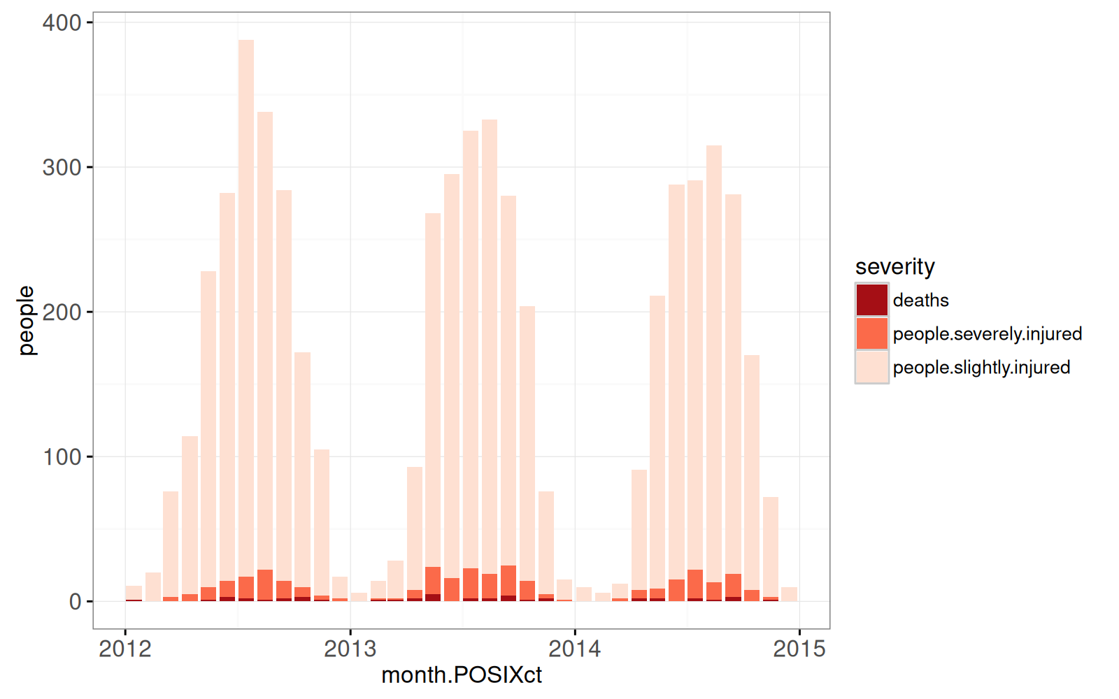
Ci-dessus, on voit le nombre de personnes décédées et blessées au fil du temps.
9.2 Visualisation interactive de la fréquence des accidents
Maintenant nous voulons comparer, pour chaque mois, les données de compteurs et d’accidents. Est-ce que nous avons plus d’accidents quand il y a plus de passages en vélo ? Pour vérifier, nous devons calculer un résumé des passages par mois avec le code ci-dessous.
              lieu mois.str passages_length passages_mean passages_sum
  1:         Berri  2009-01              31      100.3226         3110
  2:         Berri  2009-02              28      159.6786         4471
 ---
441: Totem_Laurier  2013-08              31     3162.7097        98044
442: Totem_Laurier  2013-09              18     2888.7778        51998
La sortie ci-dessus contient une ligne pour chaque combinaison de lieu et mois, avec des colonnes pour:
-
passages_length: le nombre de jours. -
passages_mean: le moyenne de passages par jour. -
passages_sum: le total nombre de passages.
On remarque que certains mois contiennent des journées manquantes. Par exemple, il n’y a que 29 jours pour Berri en avril 2009, et 18 jours pour Totem_Laurier en septembre 2013. Pour modeliser seulement les mois entiers, nous voulons enlever les mois avec jours manquants. Alors on utilise le code ci-dessous pour calculer le nombre de jours dans chaque mois :
un.jour <- 60 * 60 * 24
mois_suivant <- function(POSIXct)mois_01(POSIXct + un.jour * 31)
passages.par.mois[, jours.dans.mois := as.integer(round(difftime(
  mois_01(mois_str(mois_suivant(mois_01(mois.str)))),
  mois_01(mois.str),
  units="days"
)))][]
lieu mois.str passages_length passages_mean passages_sum
1: Berri 2009-01 31 100.3226 3110
2: Berri 2009-02 28 159.6786 4471
---
441: Totem_Laurier 2013-08 31 3162.7097 98044
442: Totem_Laurier 2013-09 18 2888.7778 51998
jours.dans.mois
1: 31
2: 28
---
441: 31
442: 30Dans la sortie ci-dessus, on voit la nouvelle colonne jours.dans.mois. Avec le code ci-dessous, on affiche seulement les mois avec jours manquants :
passages.par.mois[
  passages_length < jours.dans.mois,
  .(lieu, mois.str, passages_length, jours.dans.mois)]
lieu mois.str passages_length jours.dans.mois
1: Berri 2009-04 29 30
2: Berri 2011-11 3 30
---
22: Rachel 2013-09 18 30
23: Totem_Laurier 2013-09 18 30Nous allons exclure les données ci-dessus, en utilisant le code ci-dessous :
mois.complets <- passages.par.mois[passages_length == jours.dans.mois]Ensuite, nous faisons un tableau avec les passages et les accidents dans différents colonnes :
city.wide.complete <- mois.complets[passages_sum>0, .(
  lieux=.N,
  total.passages=sum(passages_sum)
), keyby=mois.str]
city.wide.accidents <- accidents_dt[, .(
  total.accidents=.N
), keyby=mois.str]
(scatter.not.na <- city.wide.accidents[
  city.wide.complete, nomatch=0L
][, mois.01 := mois_01(mois.str)][])
mois.str total.accidents lieux total.passages mois.01
1: 2012-01 11 7 20386 2012-01-01
2: 2012-02 19 7 26727 2012-02-01
---
17: 2013-07 315 8 916662 2013-07-01
18: 2013-08 326 8 856066 2013-08-01Dans la sortie ci-dessus, on voit une ligne pour chaque mois avec les données de compteurs et accidents. Ensuite, nous faisons un modèle linéaire pour prédire les accidents à partir des passages :
(fit <- lm(total.accidents ~ total.passages - 1, scatter.not.na))
Call:
lm(formula = total.accidents ~ total.passages - 1, data = scatter.not.na)

Coefficients:
total.passages
0.0003723 scatter.not.na[, mean(total.accidents/total.passages)][1] 0.0003847625[1] 0.0003693805Dans la sortie ci-dessus, on voit que le coefficient du modèle est proche des moyennes empiriques. Enfin, nous faisons un graphique interactif avec le code ci-dessous.
scatter.not.na[, let(
  pred.accidents = predict(fit),
  mois.français = mois_français(mois.01)
)]
animint(
  regression=ggplot()+
    theme_bw()+
    ggtitle("Accidents et passages par mois")+
    geom_line(aes(
      total.passages, pred.accidents),
      color="grey",
      data=scatter.not.na)+
    geom_point(aes(
      total.passages, total.accidents),
      clickSelects="mois.français",
      size=5,
      alpha=0.75,
      data=scatter.not.na)+
    ylab("Accidents par mois")+
    xlab("Passages par mois"),
  timeSeries=ggplot()+
    theme_bw()+
    ggtitle("Série temporelle : fréquence des accidents")+
    xlab("mois")+
    geom_point(aes(
      mois.01, total.accidents/total.passages),
      clickSelects="mois.français",
      size=5,
      alpha=0.75,
      data=scatter.not.na))
La visualisation des données ci-dessus contient deux graphiques réliés. Le graphique de gauche montre que le nombre d’accidents augmente avec le nombre de cyclistes. Le graphique de droite montre la fréquence des accidents au fil du temps.
9.3 Visualisation interactive avec carte et détails
Dans cette partie, nous allons faire une visualisation avec plusieurs composants :
- Résumé des compteurs : plan des compteurs ou min/max des mois pour chaque compteur, pour sélectionner un compteur.
- Détails d’un compteur, résumé des mois : séries temporelles par mois, pour les accidents et les données d’un compteur. Cliquer pour sélectionner un mois.
- Détails d’un compteur et d’un mois : séries temporelles par jour, pour le mois sélectionné.
9.3.1 Résumé des compteurs avec plan
Les données counter.locations contient l’emplacement géographique de chaque compteur. Pour examiner ces données, il faut d’abord convertir le nom en unicode :
(counter.locations <- data.table(montreal.bikes$counter.locations)[, .(
  lon = coord_X, lat = coord_Y,
  nom_comptage=iconv(nom_comptage, "latin1", "UTF-8"))])
lon lat nom_comptage
1: -73.58888 45.51955 Saint-Urbain
2: -73.57398 45.52741 Brebeuf
---
20: -73.58221 45.51370 Parc U-Zelt Test
21: -73.60311 45.52782 Saint-Laurent U-Zelt TestDans la sortie ci-dessus, on voit que la colonne nom_comptage indique l’emplacement, mais ce ne sont pas exactement les mêmes valeurs que la colonne lieu dans les données de passages. On utilise le code ci-dessous pour établir une correspondence entre les tableaux :
loc.name.code <- c(
  Berri1="Berri",
  Brebeuf="Brébeuf",
  CSC="Côte-Sainte-Catherine",
  Maisonneuve_1="Maisonneuve 1",
  Maisonneuve_2="Maisonneuve 2",
  Parc="du Parc",
  PierDup="Pierre-Dupuy",
  "Rachel/Papineau"="Rachel",
  "Saint-Urbain"="Saint-Urbain",
  Totem_Laurier="Totem_Laurier")
(show.locations <- counter.locations[
, lieu := loc.name.code[nom_comptage]
][!is.na(lieu)])
lon lat nom_comptage lieu
1: -73.58888 45.51955 Saint-Urbain Saint-Urbain
2: -73.57398 45.52741 Brebeuf Brébeuf
---
9: -73.58883 45.52777 Totem_Laurier Totem_Laurier
10: -73.56284 45.51613 Berri1 BerriLa sortie ci-dessus contient l’emplacement géographique pour chaque compteur. L’emplacement des compteurs est tracé ci-dessous.
map.lim <- show.locations[, lapply(.SD, range), .SDcols=c("lat","lon")]
diff.vec <- sapply(map.lim, diff)
diff.mat <- c(-1, 1) * matrix(diff.vec, 2, 2, byrow=TRUE)
scale.mat <- as.matrix(map.lim) + diff.mat
bike.paths <- data.table(montreal.bikes$path.locations)
show.paths <- bike.paths[(
  lat %between% scale.mat[, "lat"]
) & (
  lon %between% scale.mat[, "lon"]
)]
(mtl.map <- ggplot()+
   theme_bw()+
   theme(
     panel.margin=grid::unit(0, "lines"),
     axis.line=element_blank(), axis.text=element_blank(),
     axis.ticks=element_blank(), axis.title=element_blank(),
     panel.background = element_blank(),
     panel.border = element_blank())+
   coord_cartesian(xlim=map.lim$lon, ylim=map.lim$lat)+
   scale_x_continuous(limits=map.lim$lon)+
   scale_y_continuous(limits=map.lim$lat)+
   geom_path(aes(
     lon, lat,
     tooltip=TYPE_VOIE,
     group=paste(feature.i, path.i)),
     color="grey",
     data=show.paths)+
   geom_text(aes(
     lon, lat,
     label=lieu),
     clickSelects="lieu",
     data=show.locations))
Warning: Removed 96 rows containing missing values (geom_path).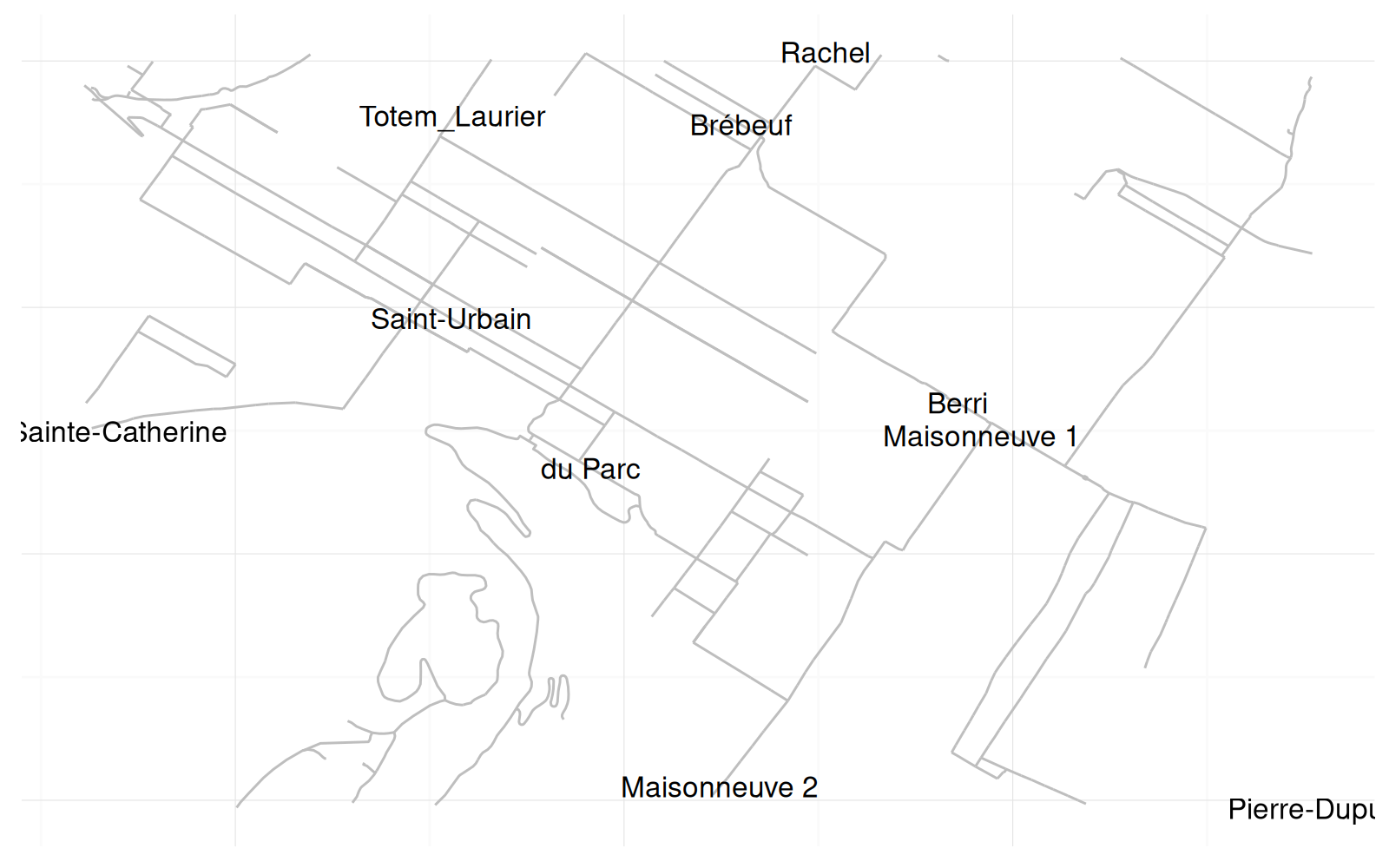
La sortie ci-dessus est un plan de Montréal, avec texte pour chacun des dix compteurs.
9.3.2 Résumé des dates extrêmes pour chaque compteur
Maintenant on calcule les dates extrêmes pour chaque compteur :
             lieu mois.01_min mois.01_max
 1:         Berri  2009-01-01  2013-09-01
 2:       Brébeuf  2009-07-01  2010-11-01
---
 9:  Saint-Urbain  2009-01-01  2010-11-01
10: Totem_Laurier  2013-02-01  2013-09-01
Dans la sortie ci-dessus, on voit une ligne pour chaque compteur, avec des colonnes pour les dates extrêmes. Le graphique ci-dessous montre la période pendant laquelle chaque compteur a fonctionné.
location.colors <- c(#dput(RColorBrewer::brewer.pal(12, "Set3"))
  "#8DD3C7", "grey50", "#BEBADA", "#FB8072", "#80B1D3", "#FDB462",
  "#B3DE69", "#FCCDE5", "#D9D9D9", "#BC80BD", "#CCEBC5", "#FFED6F")
names(location.colors) <- show.locations$lieu
seg.size <- 10
(CounterRanges <- ggplot()+
  theme_bw()+
  xlab("min/max dates")+
  ylab("source de données")+
  scale_color_manual(values=location.colors)+
  guides(color="none")+
  geom_segment(aes(
    mois.01_min, lieu,
    xend=mois.01_max, yend=lieu),
    showSelected="lieu",
    data=location.ranges,
    size=seg.size+2)+
  geom_segment(aes(
    mois.01_min, lieu,
    xend=mois.01_max, yend=lieu,
    color=lieu),
    clickSelects="lieu",
    data=location.ranges,
    size=seg.size))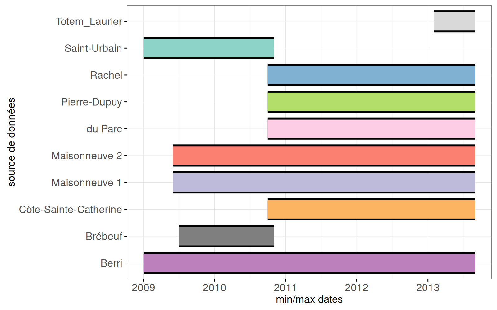
La sortie ci-dessus contient un segment pour chaque compteur. Avec le code ci-dessous, nous rajoutons un segment pour les accidents.
accidents.range <- dcast(
  data.table(lieu="accidents", accidents_dt),
  lieu ~ .,
  list(min, max),
  value.var="date")
(MonthSummary <- CounterRanges+
  geom_segment(aes(
    date_min, lieu,
    xend=date_max, yend=lieu),
    color=gravité.colors[["décès"]],
    data=accidents.range,
    size=seg.size))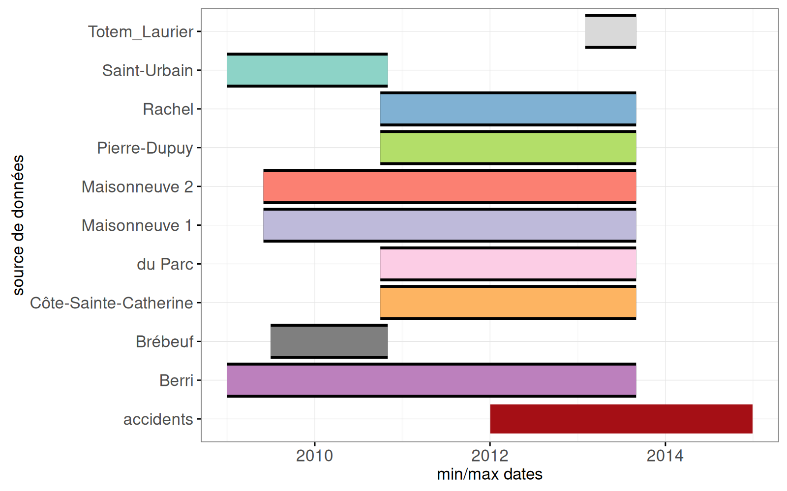
Dans la sortie ci-dessus, on voit un segment de plus (pour les accidents en bas).
9.3.3 Séries temporelles par mois
Le graphique ci-dessous présente le comptage de vélos à chaque localisation, chaque jour.
ggplot()+
  theme_bw()+
  geom_line(aes(
    date, passages, group=lieu),
    data=passages_dt)+
  scale_color_manual(values=location.colors)+
  geom_point(aes(
    date, passages, color=lieu),
    data=passages_dt)
Warning: Removed 407 rows containing missing values (geom_point).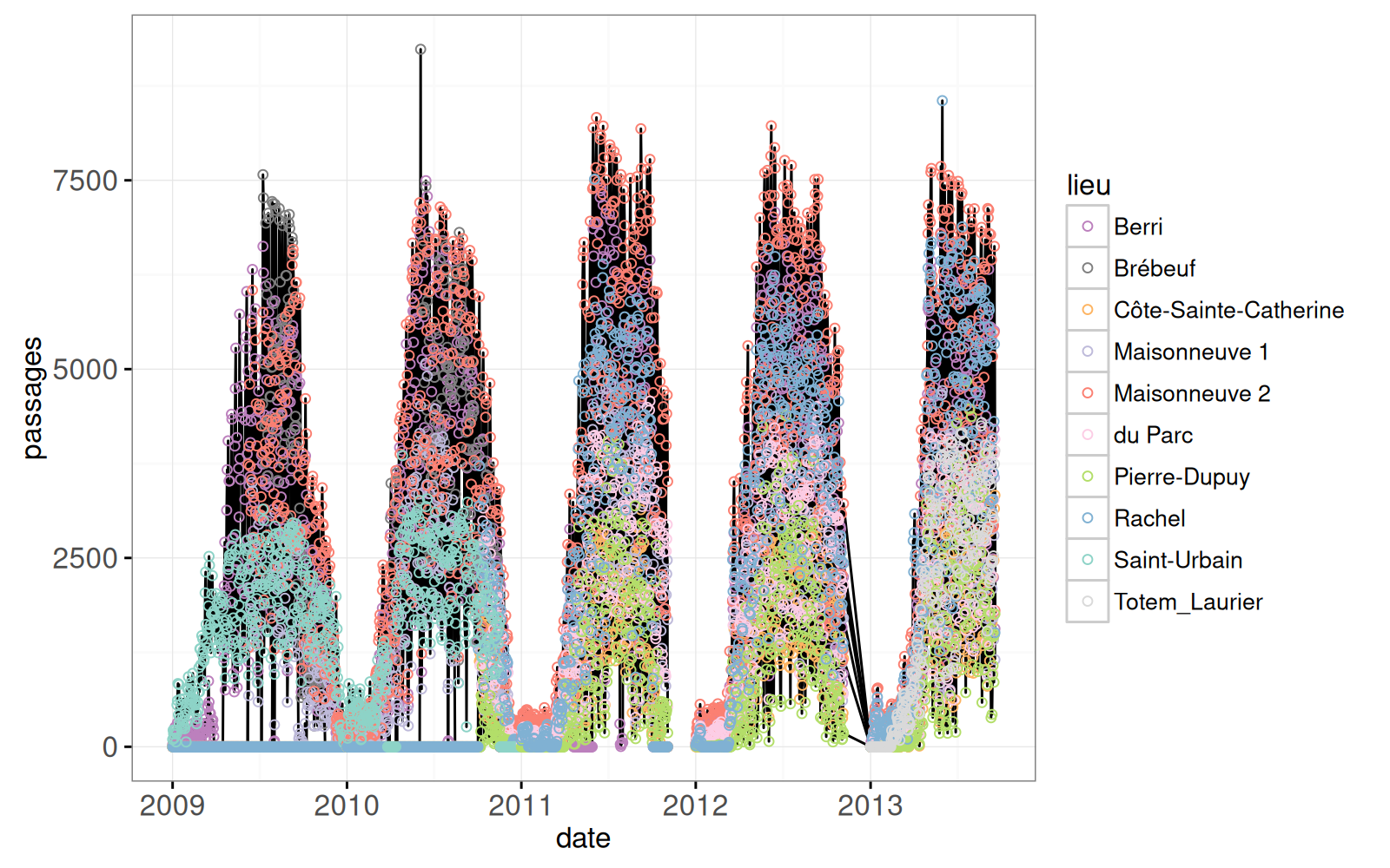
Le graphique ci-dessous reprend les mêmes données mais pour chaque mois.
FACET <- function(DT, facet)data.table(DT, facet)
COMPTEURS <- function(DT)FACET(DT, "passages/jour")
(MonthSeries <- ggplot()+
  guides(color="none")+
  theme_bw()+
  facet_grid(facet ~ ., scales="free")+
  geom_tallrect(aes(
    xmin=mois.01-15*un.jour, xmax=mois.01+15*un.jour),
    clickSelects="mois.français",
    data=mois_dt,
    alpha=1/2)+
  geom_line(aes(
    mois_01(mois.str), passages_mean, group=lieu,
    color=lieu),
    showSelected="lieu",
    clickSelects="lieu",
    data=COMPTEURS(passages.par.mois))+
  scale_color_manual(values=location.colors)+
  xlab("mois")+
  ylab(""))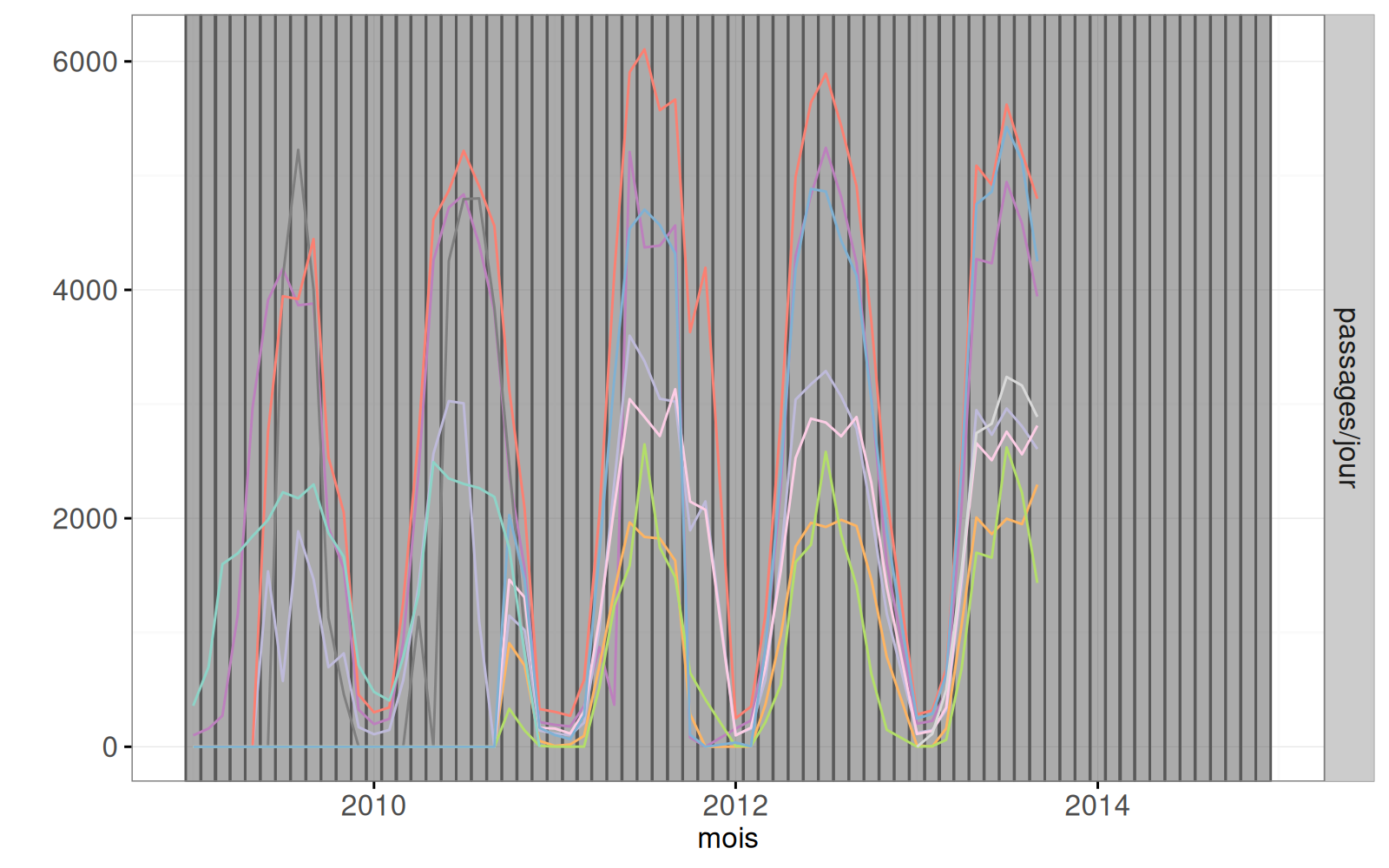
Le graphique ci-dessus contient une ligne pour chaque compteur. Dans le code ci-dessous, on rajoute deux geoms.
mois.text <- passages.par.mois[
, .SD[which.max(passages_mean)]
, by=lieu]
(MonthText <- MonthSeries+
  geom_point(aes(
    mois_01(mois.str), passages_mean, color=lieu,
    tooltip=paste(
      passages_mean, "vélos à",
      lieu, "en", mois_français(mois_01(mois.str)))),
    showSelected="lieu",
    clickSelects="lieu",
    size=5,
    data=COMPTEURS(passages.par.mois))+
  geom_text(aes(
    mois_01(mois.str), passages_mean+300,
    color=lieu, label=lieu),
    showSelected="lieu",
    clickSelects="lieu",
    data=COMPTEURS(mois.text)))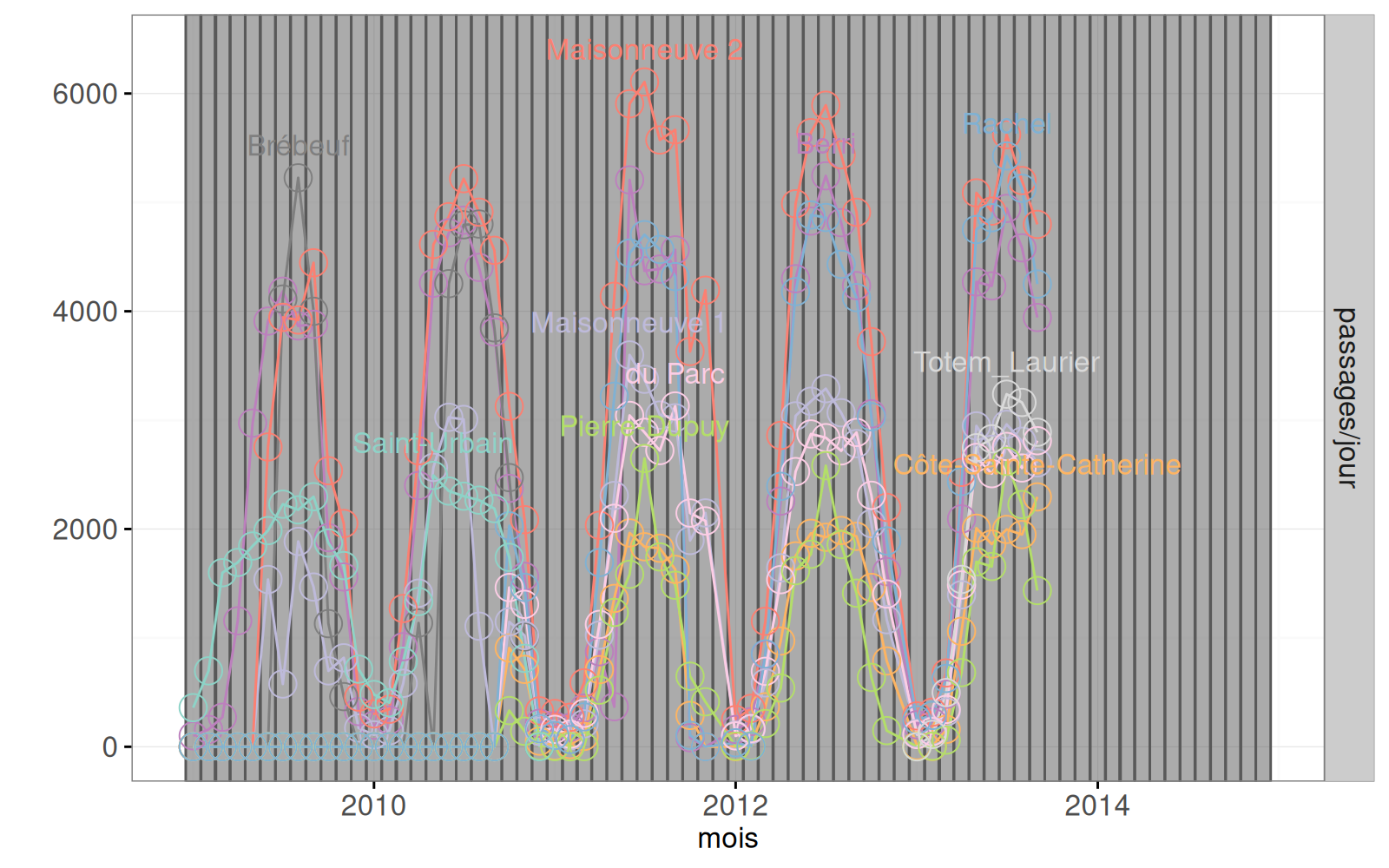
Le graphique ci-dessous rajoute les accidents.
ACCIDENTS <- function(DT)FACET(DT, "accidents")
(MonthFacet <- MonthText+
   facet_grid(facet ~ ., scales="free")+
   scale_fill_manual(
     values=gravité.colors, breaks=names(gravité.colors))+
   geom_bar(aes(
     mois_01(mois.str), personnes,
     fill=gravité),
     showSelected="gravité",
     stat="identity",
     position="identity",
     color=NA,
     data=ACCIDENTS(accidents.tall[order(-gravité)])))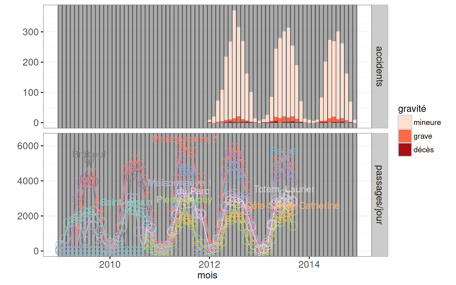
Dans la sortie ci-dessus, on voit les deux sources de données (accidents et compteurs).
9.3.4 Détails pour un mois
Dans cette partie, nous voulons faire un graphique des accidents pour chaque mois, avec un point pour chaque personne qui a eu un accident. Ci-dessous, nous classons la gravité de chaque accident en fonction du résultat le plus grave pour les personnes touchées.
gravité
mineure   grave   décès
   5262     289      44
Le résultat ci-dessus montre que les accidents avec des blessures mineures sont les plus fréquents et que les accidents avec au moins un décès sont les moins fréquents. Dans le code ci-dessous, nous faisons une colonne accident.i qui donne un numéro unique pour chaque accident dans chaque jour.
jour_du_mois <- function(POSIXct)as.integer(strftime(POSIXct, "%d"))
add_jour_mois <- function(DT)DT[, let(
  jour.du.mois = jour_du_mois(date),
  mois.français = mois_français(date))]
accidents.cumsum <- add_jour_mois(accidents_dt[
  order(date, -gravité)
][
, accident.i := seq_len(.N)
, by=date
])
ggplot()+
  theme_bw()+
  theme(panel.margin=grid::unit(0, "cm"))+
  facet_wrap("mois.str")+
  scale_fill_manual(values=gravité.colors)+
  scale_x_continuous("jour du mois", breaks=c(1, 10, 20, 30))+
  geom_point(aes(
    jour.du.mois, accident.i, fill=gravité),
    data=accidents.cumsum)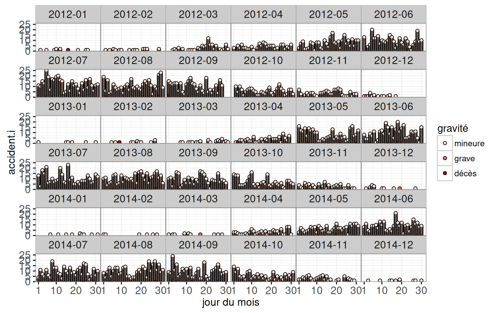
Dans la sortie ci-dessus, on voit un point pour chaque accident. Ensuite, on fait une grille de jours dans le code ci-dessous.
            date jds
   1: 2009-01-01 jeu
   2: 2009-01-02 ven
  ---
2191: 2014-12-31 mer
2192: 2015-01-01 jeu
La sortie ci-dessus contient une ligne pour chaque jour dans la période où nous avons des données. Dans le code ci-dessous, on fait un tableau pour souligner les fins de semaine.
(weekend.dt <- add_jour_mois(days.dt[
  grepl("sam|dim", jds)#windows="sam." ubuntu="sam"
])[])
date jds jour.du.mois mois.français
1: 2009-01-03 sam 3 janvier 2009
2: 2009-01-04 dim 4 janvier 2009
---
625: 2014-12-27 sam 27 décembre 2014
626: 2014-12-28 dim 28 décembre 2014La sortie ci-dessus contient une ligne pour chaque jour de fin de semaine. Ensuite, on fait un tableau qu’on va utiliser pour afficher le nom de chaque lieu.
add_jour_mois(passages_dt)
(jour.text <- passages_dt[
, .SD[which.max(passages)]
, by=.(lieu, mois.français)])
lieu mois.français date mois.str passages
1: Berri janvier 2009 2009-01-11 05:00:00 2009-01 318
2: Berri février 2009 2009-02-18 05:00:00 2009-02 326
---
441: Totem_Laurier août 2013 2013-08-21 04:00:00 2013-08 4293
442: Totem_Laurier septembre 2013 2013-09-18 04:00:00 2013-09 3921
lieu.lines jour.du.mois
1: Berri 11
2: Berri 18
---
441: Totem\nLaurier 21
442: Totem\nLaurier 18La sortie ci-dessus contient le jour avec le plus de passages, pour chaque lieu et mois. Ensuite, le code ci-dessous fait un graphique de passages par jour sur les compteurs.
(DaysCompteurs <- ggplot()+
  geom_tallrect(aes(
    xmin=jour.du.mois-0.5, xmax=jour.du.mois+0.5,
    key=paste(date)),
    showSelected="mois.français",
    fill="grey",
    color="white",
    data=weekend.dt)+
  guides(color="none", fill="none")+
  theme_bw()+
  facet_grid(facet ~ ., scales="free")+
  geom_line(aes(
    jour.du.mois, passages, group=lieu,
    key=lieu, color=lieu),
    showSelected=c("lieu", "mois.français"),
    clickSelects="lieu",
    chunk_vars=c("mois.français"),
    data=COMPTEURS(passages_dt))+
  scale_color_manual(values=location.colors)+
  ylab("")+
  geom_point(aes(
    jour.du.mois, passages, color=lieu,
    key=paste(jour.du.mois, lieu),
    tooltip=paste(
      passages, "cyclistes à",
      lieu, "en",
      date)),
    showSelected=c("lieu", "mois.français"),
    clickSelects="lieu",
    size=5,
    chunk_vars=c("mois.français"),
    fill="white",
    data=COMPTEURS(passages_dt)))
Warning: Removed 407 rows containing missing values (geom_point).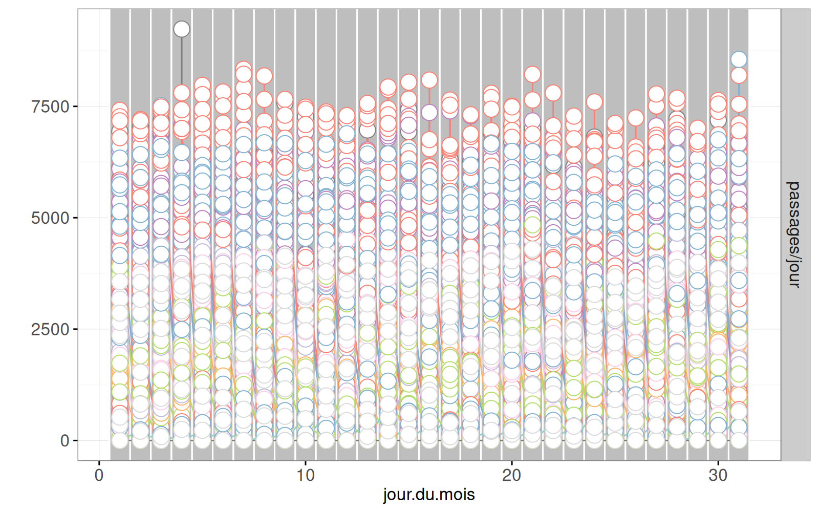
La sortie ci-dessus affiche les données des compteurs, avec trop de données car le graphique statique ne prend pas en compte du mot-clé showSelected. Le code ci-dessous rajoute les données d’accidents.
(DaysFacet <- DaysCompteurs+
   scale_fill_manual(
     values=gravité.colors, breaks=names(gravité.colors))+
   geom_text(aes(
     15, 23, label=mois.français, key=1),
     showSelected="mois.français",
     data=ACCIDENTS(mois_dt))+
   scale_x_continuous("jour du mois", breaks=c(1, 10, 20, 30))+
   geom_point(aes(
     jour.du.mois, accident.i,
     key=paste(date.str, accident.i),
     fill=gravité),
     showSelected=c("gravité","mois.français"),
     size=4,
     chunk_vars=c("mois.français"),
     data=ACCIDENTS(accidents.cumsum)))
Warning: Removed 407 rows containing missing values (geom_point).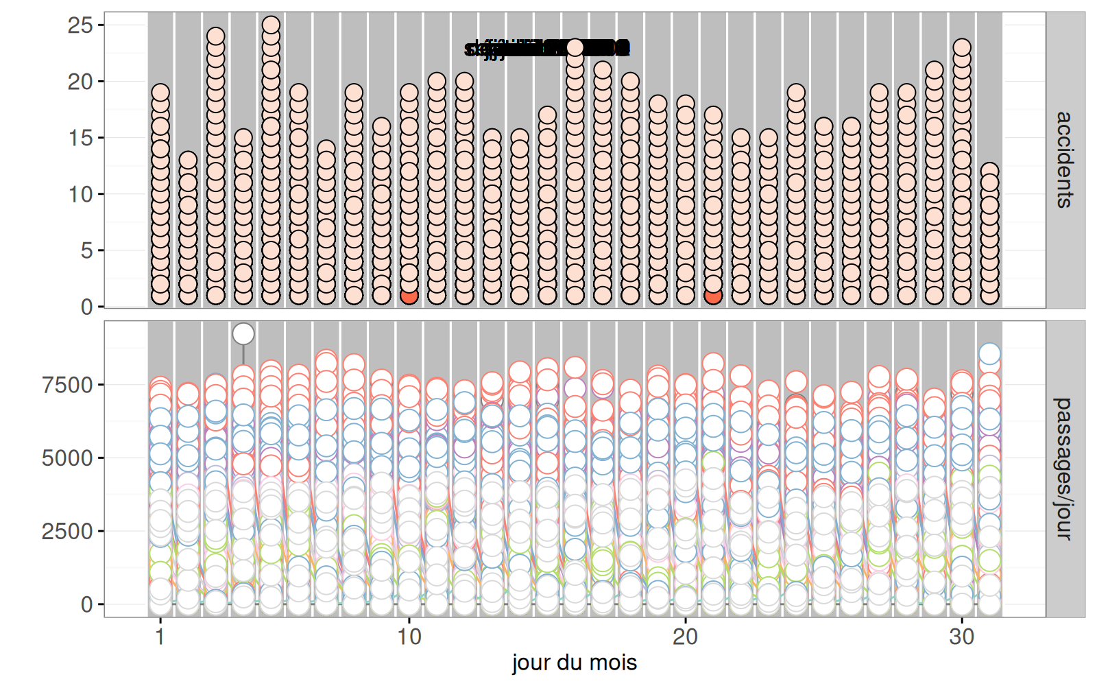
La sortie ci-dessus contient les deux séries temporelles (accidents et compteurs).
9.3.5 Graphique interactif
Enfin, le code ci-dessous combine tous les graphiques.
animint(
  MonthFacet+
    ggtitle("Toutes les données, choisir mois"),
  DaysFacet+
    ggtitle("Mois sélectionné (week-ends en gris)")+
    geom_label_aligned(aes(
      jour.du.mois, passages+1500, color=lieu, label=lieu,
      key=lieu),
      showSelected=c("lieu", "mois.français"),
      clickSelects="lieu",
      data=COMPTEURS(jour.text))+
    theme_animint(last_in_row=TRUE),
  MonthSummary+theme_animint(width=450, height=250),
  mtl.map+theme_animint(height=250),
  selector.types=list(severity="multiple"),
  duration=list(mois.français=2000),
  first=list(
    lieu="Maisonneuve 2",
    mois.français="juillet 2012"))
La sortie ci-dessus contient 4 graphiques :
- En haut à gauche : séries temporelles avec résumé pour chaque mois.
- En haut à droite : séries temporelles pour le mois sélectionné.
- En bas à gauche : le min et max dates pour chaque source de données.
- En bas à droite : lieux des compteurs sur le plan de Montréal.
9.4 Résumé du chapitre et exercices
Nous avons vu plusieurs graphiques pour visualiser les séries temporelles en rapport avec les vélos de Montréal.
Exercices :
- Faire
lieuune variable à sélection multiple. - Sur la carte, dessinez un cercle avec
aes(color=lieu)pour chaque compteur, dont la taille varie en fonction des passages dans le mois sélectionné. - Sur le graphique
MonthSummary, ajoutez rectangles en arrière-plan pour sélectionner le mois. - Supprimez le graphique
MonthSummaryet ajoutez une visualisation similaire dans un troisième panneau de l’écran dans le graphiqueMonthFacet. Astuce : utilisetheme_animint(rowspan=2). - Dans
DaysFacet, utilisezaes(tooltip)avec quelques détails pour chaque accident (addresse, nombre de personnes, etc).
Dans le chapitre 10, nous vous expliquerons comment visualiser le modèle d’apprentissage automatique des K-voisins les plus proches.